Trust Region Policy Optimisation (TRPO)

Policy Gradient methods are quite popular in reinforcement learning and they involve directly learning a policy $\pi$ from sampled trajectories. We generally run gradient ascent on our networks to take a step in the direction that maximises our reward but overconfidence in our steps can lead to poor performance. Sometimes even small steps in parameter space $\theta$ can lead to policies that lead to extremely different outcomes from our policy network. TRPO is an iterative procedure for optimising policies, with guaranteed monotonic improvement. It is similar to natural policy gradient methods and is effective for optimising large nonlinear policies such as neural networks. Despite its approximations that deviate from the theory, TRPO tends to give monotonic improvement, with little tuning of hyperparameters.
This post assumes basic knowledge of policy gradient methods, a refresher on this topic can be found here.

Challenges of Policy Gradient Methods

The gradient in the policy gradient algorithm is

where $g$ is the gradient. Here we’re taking the first order derivative which assumes that the surface of our function is relatively flat when in fact it could be highly curved. A large step on a highly curved surface could lead to a drastically different policy which is extremely bad during training, meanwhile if we take too small a step our network will take too long to converge.

For example, if our old policy is taking a path that is too close to the edge of a cliff, a large step during gradient ascent could lead to a new policy that veers off the cliff. The performance collapses and it will take a long time to recover if ever.

We should constraint the policy change every iteration. In regular gradient descent the magnitude of the gradient x $\alpha$ decides our step size. It can be seen as taking a step of length $\alpha$|g| from our current parameters which would be a circle where the length of the step is equal to the radius of the circle. The direction in which we move is given by the gradient. Thus we’re imposing a constraint in parameter space to select a set of parameters that are within this circle, when instead we should be imposing a constraint in the distribution space. We can do this by applying a constraint on the KL divergence between our new policy and our current policy.

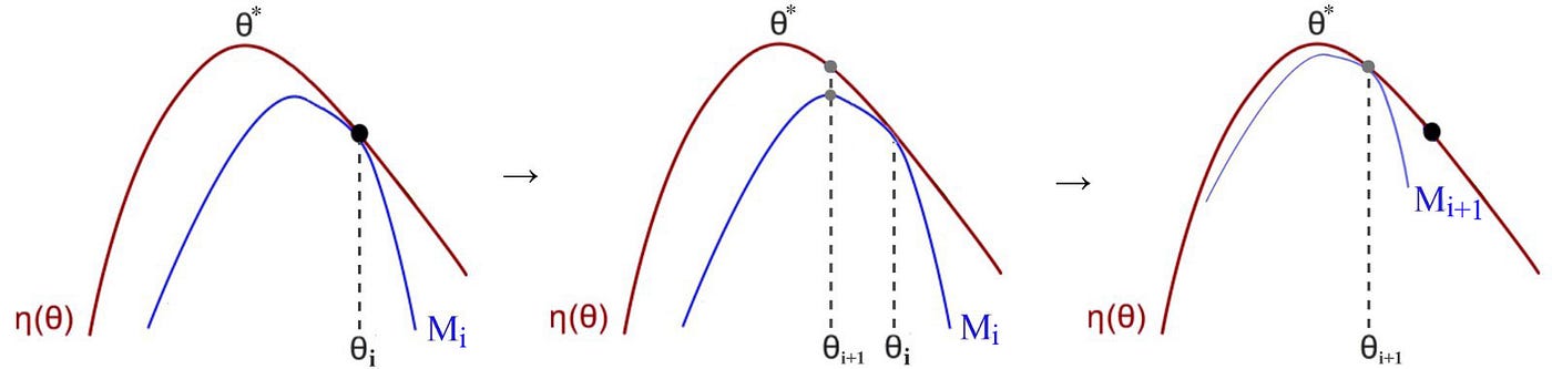
Minorize-Maximization MM algorithm

The MM algorithm constructs a lower bound for our expected reward at each iteration and then proceeds to maximise this lower bound with respect to $\theta$. We do this iteratively until we converge to the optimal policy. In TRPO we will construct a lower bound which we’ll call the surrogate advantage/function and then optimise our parameters w.r.t it.

Key Equations

Let’s define a surrogate function which is a measure of how our new policy $\pi_{\theta}$ performs with respect to our old policy $\pi_{\theta_{k}}$ using samples generated by our old policy.

$L(\theta_{k}, \theta) = argmax_{\theta} E_{s,k \sim \pi_{\theta_{k}}} [ \frac{\pi_{\theta}(a|s)}{\pi_{\theta_{k}}(a|s)} A^{\pi_{\theta_{k}}}(s,a)]$

Our goal is to maximise this lower bound under the following constraint

and

is the average KL divergence between policies across states visited by the old policy.

$D_{KL}(\theta||\theta_{k}) = E_{s \sim \pi_{\theta_{k}}}[D_{KL}(\pi_{\theta}(.|s)||\pi_{\theta_{k}}(.||s))]$

The theoretical TRPO update isn’t the easiest to work with, so TRPO makes some approximations to get an answer quickly. We Taylor expand the objective and constraint to leading order around $\theta_{k}$:

$L(\theta_{k},\theta) \approx g^{T}( \theta - \theta_{k})$

$D_{KL}(\theta||\theta_{k}) \approx \frac{1}{2} ( \theta - \theta_{k})^{T} H ( \theta - \theta_{k})$

resulting in an approximate optimisation problem,

$\theta_{k} = argmax_{\theta} g^{T} ( \theta - \theta_{k})$

$s.t. \quad \frac{1}{2} ( \theta - \theta_{k})^{T} H ( \theta - \theta_{k}) \le \delta$

where H is the hessian of the sample average KL divergence. It is also known as the Fisher information matrix. The gradient $g$ of the surrogate function with respect to $\theta$, evaluated at $\theta = \theta_{k}$ is exactly equal to the policy gradient $\nabla_{\theta}J(\pi_{\theta})$.

This approximate problem can be analytically solved by the methods of Lagrangian duality, yielding the solution:

$\theta_{k+1} = \theta_{k} + \alpha H^{-1} g$

This is the natural gradient for our policy network. We substitute $\alpha$ as

$\theta_{k+1} = \theta_{k} + \sqrt{ \frac{2 \delta}{g^{T} H^{-1} g}} H^{-1} g$

The above algorithm is calculating the exact natural policy gradient. The problem is that, due to the approximation errors introduced by the Taylor expansion, this may not satisfy the KL constraint, or actually improve the surrogate advantage. TRPO adds a modification to this update rule: a backtracking line search,

$\theta_{k+1} = \theta_{k} + \alpha^{j} \sqrt{ \frac{2 \delta}{g^{T} H^{-1} g}} H^{-1} g$

where $\alpha \space \epsilon \space (0,1)$ is the backtracking coefficient, and $j$ is the smallest non-negative number such that $\pi_{\theta_{k}}$ satisfies the KL constraint and produces a positive surrogate function.

Lastly, computing and storing the matrix inverse, $H^{-1}$ is painfully expensive when dealing with neural network policies with 1000’s or millions of parameters. TRPO sidesteps this issue by using the conjugate gradient method for calculating $H^{-1}$.

Fisher Information

Fisher information is the second derivative of KL divergence

$F_{\pi_{\theta}} = E_{\pi_{\theta}}[ \nabla_{\theta} log(\pi_{\theta}(a|s) \space \nabla_{\theta} log(\pi_{\theta}(a|s)^{T} ]$

It contains information about the curvature the function surface. Fisher Information gives us the local distance between distributions. Intuitively, it gives the change in the distribution for a small change in parameters.

Exploration vs Exploitation

TRPO trains a stochastic policy in an on-policy way. This means that it explores by sampling actions according to the latest version of its stochastic policy. The amount of randomness in action selection depends on both initial conditions and the training procedure. Over the course of training, the policy typically becomes progressively less random, as the update rule encourages it to exploit rewards that it has already found. This may cause the policy to get trapped in local optima.

Psuedocode

TRPO Shortcomings

TRPO minimizes the quadratic equation to approximate the inverse of H

But, for each model parameter update, we still need to compute H. This hurts scalability:

• Computing H is expensive
• It requires a large batch of rollouts to approximate H accurately.