Policy Gradients

The reinforcement learning objective is to find a behaviour or policy that helps the agent maximize the reward obtained from the environment. Policy gradient methods directly represent the policy $\pi$, generally using a function parameterized by $\theta$. The goal can be represented as

The parameters $\theta$ belong to the policy network which in the simplest case would be some neural network that generates a vector of logits of length A where A is the number of actions. These logits are passed through a softmax function which generates a distribution over the actions. we can write our objective function for this network as

$J(\theta) = E_{\tau \sim \pi_{\theta}(\tau)}[r(\tau)] = \int \pi_{\theta}(\tau)r(\tau)d\tau$

$\nabla_{\theta} J(\theta) = \int \nabla_{\theta}\pi_{\theta}(\tau)r(\tau)d\tau = \int \pi_{\theta}(\tau) \nabla_{\theta}log(\pi_{\theta}(\tau))r(\tau)d\tau$

$\nabla_{\theta} J(\theta) = E_{\tau \sim \pi_{\theta}(\tau)}[\nabla_{\theta}log(\pi_{\theta}(\tau))r(\tau)]$

We substitute $\nabla_{\theta}\pi_{\theta}(\tau)$ as $\pi_{\theta}(\tau) \nabla_{\theta}log(\pi_{\theta}(\tau))$ and our new representation is still an expectation. This is called the log derivative trick. This enables us to easily make use of the auto-differentiation packages provided to us because the gradient $\nabla_{\theta}log(\pi_{\theta}(\tau))$ is similar to gradient generated by networks with softmax and crossentropy loss. The probability of a trajectory can be decomposed as

$\pi_{\theta}(\tau) = p(s_{1})\prod \pi_{\theta}(s_{t} , a_{t}) p(s_{t+1}|s_{t} , a_{t})$

where $p(s_{1})$ is the distribution over the initial states which means that

$log(\pi_{\theta}(\tau)) = log(p(s_{1}))+\sum (log(\pi_{\theta}(s_{t} , a_{t})) + log(p(s_{t+1}|s_{t} , a_{t})))$

The gradient can then be written as

$\nabla_{\theta} J(\theta) = E_{t \sim \pi_{\theta}(\tau)}[\nabla_{\theta}log(\pi_{\theta}(\tau))r(\tau)]$

$\nabla_{\theta}log(\pi_{\theta}(\tau)) = \nabla_{\theta} log(p(s_{1}))+\sum (\nabla_{\theta} log(\pi_{\theta}(s_{t} , a_{t})) + \nabla_{\theta} log(p(s_{t+1}|s_{t} , a_{t})))$

$\nabla_{\theta}log(\pi_{\theta}(\tau)) = \sum \nabla_{\theta} log(\pi_{\theta}(s_{t} , a_{t}))$

$\nabla_{\theta} J(\theta) = E_{t \sim \pi_{\theta}(\tau)}[(\sum \nabla_{\theta} log(\pi_{\theta}(s_{t} , a_{t})))(\sum r(s_{t} , a_{t}))]$

Thus we can write our gradient update as $\theta \larr \theta + \alpha \nabla_{\theta} J(\theta)$ and use our preferred optimiser to run gradient ascent

REINFORCE Algorithm

REINFORCE (Monte-Carlo policy gradient) relies on an estimated return by Monte-Carlo methods using episode samples to update the policy parameter $\theta$. The Monte-Carlo return $G_{t}$ is computed as $G_{t} = \sum_{t}^{T} r(s_{t},a_{t})$. The Monte-Carlo return for a state s_t does not include the rewards for the previous states. The Algorithm is as follows:

1. Sample {$\tau^{i}$} from $\pi_{\theta}(s_{t} , a_{t})$ (run policy)
2. $\nabla_{\theta} J(\theta) \approx \sum_{i}[(\sum_{t} \nabla_{\theta} log(\pi_{\theta}(s_{t}^{i} , a_{t}^{i})))G_{t}^{i}]$
3. $\theta = \theta + \alpha \nabla_{\theta} J(\theta)$

Note: We’ve taken $G_{t}$ as $\sum_{t}^{T} r(s_{t},a_{t})$ and ignore the rewards generated from $t’=1$ to $t’=t$. This is the property of causality. We do not want previously generated rewards to determine the importance of a given state.

Compare with Maximum Likelihood Estimation

If we simply run MLE on the obtained trajectories then our gradient is
$\nabla_{\theta} J(\theta) = E_{t \sim \pi_{\theta}(\tau)}[\sum \nabla log(\pi_{\theta}(s_{t} , a_{t}))]$

So what’s different? To put it simply, the Monte-Carlo return $G_{t}$ gives importance to the gradients that generate high returns and less importance to the gradients that give us low returns. When $G_{t}$ is high we take larger steps in the direction of the corresponding gradient, and when $G_{t}$ is negative we take a step in the direction that reduces the chances of picking those actions. So we give importance to good actions and penalise bad actions.

What is wrong with our approach so far?

• The above method has high variance. The returns $G_{t}$ may not be the same for a given state each time due to the stochastic nature of our environment. We can thus get noisy estimates of the reward and this can lead to high variance. Monte-Carlo estimates have no bias but high variance.
• If our return $G_{t}$ is always positive then we’ll end up increasing the probability of every trajectory regardless of how good it is. Let’s understand this with an example.
  • Let’s assume we’re in an environment where for a given state $s$ the best action returns a value of 1000 while the worst action returns a value of 950.
  • Ideally we should increase mass of the distribution over the policy at the area of the best action. But since the returns for all actions were large positive numbers the algorithm will try to increase the mass of the distribution over all the actions.
  • We should only be favouring actions that are better than average.

Improving Policy Gradients

Using Value Function Approximators

One way of fixing the variance problem of the Monte-Carlo estimates is to run many trajectories and average them out while calculating our gradient, but increasing the batch size becomes computationally more expensive. What if we use a separate network $Q_{\phi}(s, a)$ parametrized by $\phi$ to approximate our action value function. We can update our estimate of $Q_{\phi}(s,a)$ each time we run our training loop and then plug it into the gradient update equation instead of $G_{t}$ while running the gradient update step.

The updates will look something like this:

$\phi = \phi - 0.5\alpha \nabla[\frac{1}{N}\sum_{t}^{T}(Q_{\phi}(s_{t}, a_{t}) - G_{t})^{2}]$

$\phi = \phi - \alpha[\frac{1}{N}\sum_{t}^{T}(Q_{\phi}(s_{t}, a_{t}) - G_{t})\nabla Q_{\phi}(s_{t}, a_{t})]$

$\nabla_{\theta} J(\theta) \approx \sum_{i}[(\sum_{t} \nabla log(\pi_{\theta}(s_{t}^{i} , a_{t}^{i})))Q_{\phi}(s_{t}, a_{t})]$

$\theta = \theta + \alpha \nabla_{\theta} J(\theta)$

Introducing Baselines

Although value function approximation solves the problem of high variance, the 2nd problem mentioned in the above section has yet to be solved. We want to increase the likelihood of choosing actions that are better than average and reduce the probability of choosing the actions that are worse than average. The simplest way to do this is to subtract some value $b$ from our return. $b$ represents the average return expected from a trajectory run from that state and is called the baseline.

The gradient can be written as

$\nabla_{\theta} J(\theta) \approx \sum_{i}[(\sum_{t} \nabla log(\pi_{\theta}(s_{t}^{i} , a_{t}^{i})))(Q_{\phi}(s_{t}, a_{t}) - b)]$

Here we’ve used $Q_{\phi}(s_{t}, a_{t})$ as the state action value function but you can also plug in the Monte-Carlo return $G_{t}$. By subtracting $b$ from $Q_{\phi}(s_{t}, a_{t})$ we will only increase the probability of choosing actions that generate return greater than $b$ and reduce the probability of choosing actions that generate return lesser than $b$.

We can define the advantage function as

$A^{\pi} = Q_{\phi}(s_{t}, a_{t}) - b$

which gives us the advantage of picking a certain action as opposed to any other action.

The gradient can be written as

$\nabla_{\theta} J(\theta) \approx \sum_{i}[(\sum_{t} \nabla log(\pi_{\theta}(s_{t}^{i} , a_{t}^{i})))A^{\pi}(\tau)]$

Alternatively you can use the Monte-Carlo returns as the expected return from a state and use the $V_{\phi}(s)$ as the baseline.

Note Subtracting our baseline from expected return does not introduce any bias. it only reduces the variance

$E[\nabla_{\theta} log(\pi_{\theta}(\tau)b] = \int \pi_{\theta}(\tau) \nabla_{\theta}log(\pi_{\theta}(\tau))bd\tau = \int \nabla_{\theta}\pi_{\theta}(\tau)bd\tau$

$= b\int \nabla_{\theta}\pi_{\theta}(\tau)d\tau = b\nabla_{\theta}\int \pi_{\theta}(\tau)d\tau = b\nabla_{\theta}(1) = b(0) = 0$

Hence proving that no bias is introduced by the subtraction of the baseline

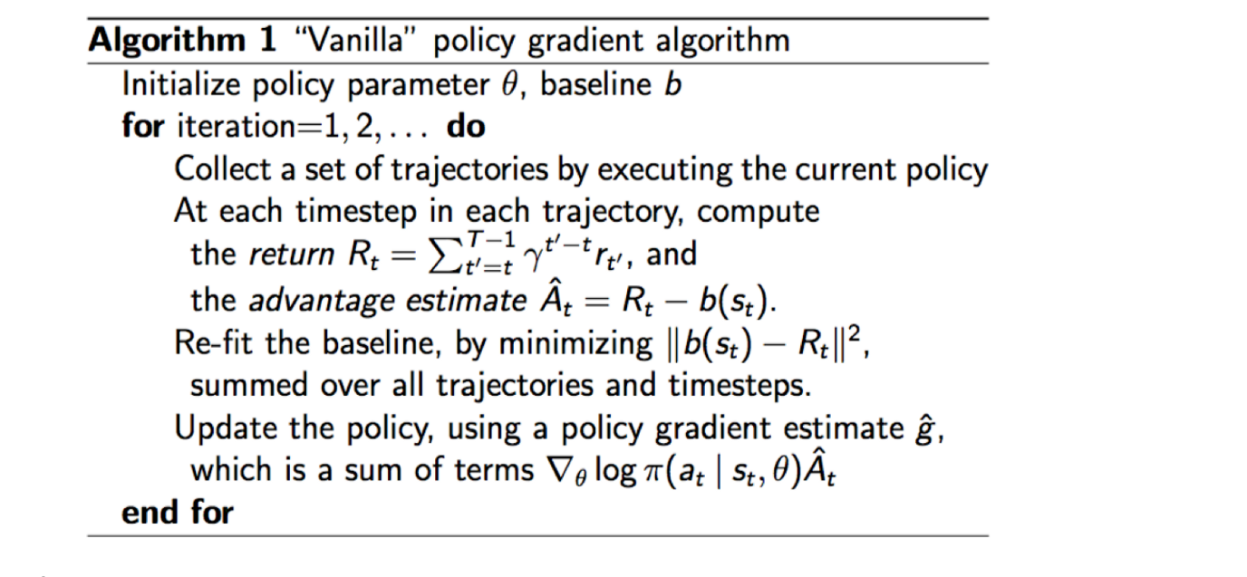
Vanilla Policy gradient Algorithm

The following is the Vanilla policy gradient algorithm, it is using the Monte-Carlo returns for estimating return. It is using the value function $V_{\phi}(s)$ as the baseline. $V_{\phi}(s)$.

Off-Policy Policy Gradient

So far the methods introduced have all been On-policy. Since neural networks change a little bit with each gradient step this can be extremely inefficient. It would be very useful if we could use the trajectories sampled from previous policies instead of discarding them.

Importance Sampling

Importance sampling helps us use trajectories sampled from previous policies while training. It’s derived as follows:

$E_{x \sim p(x)}[f(x)] = \int p(x) f(x) dx$

$= \int q(x) \frac{p(x)}{q(x)}f(x) dx$

$= E_{x \sim q(x)}[\frac{p(x)}{q(x)}f(x)]$

Thus we can write the above expectation over p(x) as an expectation over q(x).

Deriving the Policy Gradient with Importance Sampling

$\theta^{*} = argmax_{\theta}J(\theta)$

$J(\theta) = E_{\tau \sim \pi_{\theta}(\tau)}[r(\tau)]$

Can we estimate the value of some new parameters $\theta’$ using the trajectories generated by $\theta$?

$J(\theta') = E_{\tau \sim \pi_{\theta}(\tau)}[ \frac{\pi_{\theta'}(\tau)}{\pi_{\theta}(\tau)} r(\tau)]$

Thus the gradient becomes

$\nabla_{\theta'} J(\theta') = E_{\tau \sim \pi_{\theta}(\tau)}[ \frac{\nabla_{\theta'}\pi_{\theta'}(\tau)}{\pi_{\theta}(\tau)} r(\tau)]$

$\nabla_{\theta'} J(\theta') = E_{\tau \sim \pi_{\theta}(\tau)}[ \frac{\pi_{\theta'}(\tau)}{\pi_{\theta}(\tau)} \nabla_{\theta'} log(\pi_{\theta'}(\tau)) r(\tau)]$

Policy gradient with automatic differentiation

Here’s an example of Tensorflow pseudocode for policy gradients:

Maximum likelihood:

# Given: 
# actions - (N*T) x Da tensor of actions 
# states - (N*T) x Ds tensor of states 
# Build the graph:

logits = policy.predictions(states)
negative_likelihoods = tf.nn.softmax_cross_entropy_with_logits(labels=actions, logits=logits)
loss = tf.reduce_mean(negative_likelihoods)
gradients = loss.gradients(loss, variables)

Policy Gradient

# Given: 
# actions - (N*T) x Da tensor of actions 
# states - (N*T) x Ds tensor of states 
# q_values – (N*T) x 1 tensor of estimated state-action values 
# Build the graph:

logits = policy.predictions(states)
negative_likelihoods = tf.nn.softmax_cross_entropy_with_logits(labels=actions, logits=logits)
weighted_negative_likelihoods = tf.multiply(negative_likelihoods, q_values)
loss = tf.reduce_mean(weighted_negative_likelihoods)
gradients = loss.gradients(loss, variables)

Review

• Policy gradient is on-policy. The off-policy variant can be derived using importance sampling.
• Remember that the gradient is high variance. Consider larger batch sizes and using baselines to reduce the variance.
• Tweaking learning rates is very hard, Adaptive step size rules like ADAM can be ok-ish.